Result Interpretation
Proper interpretation of hcprequestanalytics results requires some good knowledge about how HCP works, as well as about http, networking and client behaviour. The information in this chapter hopefully helps understanding the results a bit.[1]
Load distribution
You can use the node_* queries to find out how load is distributed across the nodes.
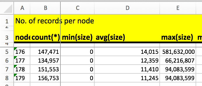
As the example shows, the load distribution is OK so far. A slight deviation is normal due to DNS (and/or loadbalancer) behaviour.
Due to the nature of HCP, you’ll want all load to be distributed evently across all available HCP Nodes.
Who’s generating load
Often, it is of interest to find out who exactly is generating load towards HCP. The clientip_* queries are your friend in this case:
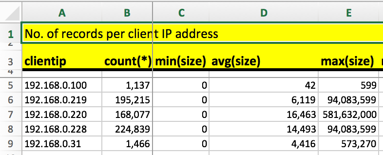
You will still need to map the IP-addresses to your clients, as usual.
Request size
All versions of HCP prior to version 8 are logging request sizes for GET requests (and some POST requests), only. That’s why often enough a request size of zero is reported for everything else.
That of course has its implications regarding throughput (Bytes/sec), which can only be calculated for requests with sizes > zero.
Latency
The latency column, seen in the result of many queries, state what is called the HCP internal latency. That means, it talks about the time passed between the clients’ request being received by HCP until the last byte of HCPs answer was sent back to the client. During this time, things like fetching the object from the backend storage, de-compression and/or de-cryption will take place, adding to the overall time needed for sending or receiving the objects data itself.
The latency value itself doesn’t tell too much, as long it’s not put into relation with the size of the request. In addition, latency created by the network and even the client will go into this value, as long as these latencies take place while the request is between the two states mentioned in the beginning.
That means that a huge latency most likely isn’t an issue with huge objects, but might be with small ones.
Throughput
Throughput, mentioned as Bytes/sec in some of the queries’ results, is a simple calculation of size devided by latency. It does not necessarily tell you the network throughput for a single object, as the latency also takes in account the time needed to de-crypt or un-compress the object before delivery to the client, for example.
Interpretation of percentiles
A percentile (or a centile) is a measure used in statistics indicating the value below which a given percentage of observations in a group of observations fall. For example, the 20th percentile is the value (or score) below which 20% of the observations may be found.[2]
The percentile_* queries try to make use of this by presenting a wide range of percentiles for size, latency and Bytes/sec (see the Throughput section!). Basically, it will tell you how your values are distributed within the entire range of 100% of the data.
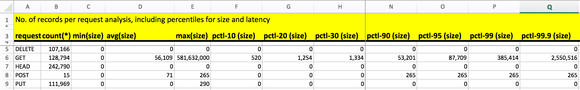
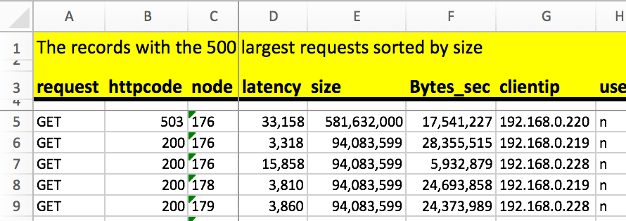
Let’s take row 6 as an example - it tells that the GET request with the
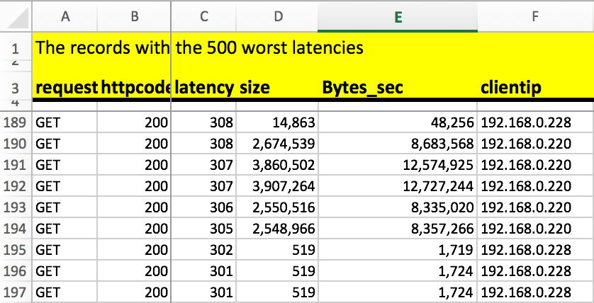
hugest size was 581,632,000 bytes. But it also tells that 99.9% of the GET
requests are 2,550,516 Bytes or smaller (cell Q6). This lets us know that
the max(size) value is just a peak, appearing in the highest 0.1% of the
requests. Looking at the 500_largest_size query result will proof that:
This gives a good overview, but still needs to be taken in relation with other parameters - for example, if you have overall high latency, you might also have overall huge request sizes…
Footnotes
| [1] | All queries referenced in this chapter are based on the built-in queries. |
| [2] | Taken from the Percentile article at Wikipedia |
